Model development

This section walk you through the creation of a mechanistic model from text.

How to use

pasmopy.Text2Model is a useful class to build an ordinary differential equation (ODE) model from a text file describing biochemical systems.

The text file you need to prepare can be divided into three parts:

Reaction layer
Observable layer (Prefix: @obs)
Simulation layer (Prefix: @sim)

Note

To write a comment, simply put the hash mark # before your desired comment.

# This is a comment.

Reaction layer

description | parameters | initial conditions

In the reaction layer, you need to describe biochemical reactions. Each reaction described in the line number i will be converted into i^th rate equation. To specify parameters or initial conditions, you can put those information after |.

If you don’t specify parameters/initial_conditions, they are initialized to 1 and 0, respectively, and the parameter values will be estimated from experimental data.
If you want to set a parameter value to 1 and don’t want to estimate, you can add const prefix:

# The Hill coefficient is fixed to 1.
TF transcribes mRNA | const n=1

You can impose parameter constraints by specifying line number in the parameter section.

# Nucleocytoplasmic Shuttling of DUSP
DUSPc translocates from the cytoplasm to the nucleus <--> DUSPn
pDUSPc translocates from the cytoplasm to the nucleus <--> pDUSPn |2|

In the example above, you can assume that import and export rates were identical for DUSP (line 2) and pDUSP (line 3).

If the amount of a model species should be held fixed (never consumed) during simulation, you can add fixed prefix:

# [Ligand] will be held fixed to 10.0 during simulation
Ligand binds Receptor <--> LR | kf = 1e-6, kr = 1e-1 | fixed Ligand = 10.0

To describe more complex rate equations, you can use @rxn prefix:

@rxn Reactant --> Product: define rate equation here

Please also refer to the following example: cfos_model

Note

The available rules can be found at https://biomass-core.readthedocs.io/en/latest/api/reaction_rules.html.

You can also supply your own terminology in a reaction rule via:

from pasmopy import Text2Model

# Supply "releases" to the reaction rule: "dissociate"
mm_kinetics = Text2Model("michaelis_menten.txt")
mm_kinetics.register_word({"dissociate": ["releases"]})
# Now you can use "releases" in your text, e.g., 'ES releases E and P'
mm_kinetics.convert()

Observable layer (Prefix: `@obs`)

In the observable layer, you need to specify biomass.observables, which can correlate model simulations and experimental measurements. You can create an observable by using model parameters (p) and species (u). For example, if the total amount of SOS bound to EGFR should be the sum of RGS (EGFR-Grb2-SOS) and RShGS (EGFR-Shc-Grb2-SOS) complexes in your model, then you can write as follows:

@obs Total_SOS_bound_to_EGFR: u[RGS] + u[RShGS]

Simulation layer (Prefix: `@sim`)

In the simulation layer, you can set simulation conditions, e.g, the simulation time span, the initial concentration of model species, etc.

Example:

@sim tspan: [0, 120]
@sim unperturbed: init[EGF] = 0
@sim condition EGF20nM: init[EGF] = 680
@sim condition EGF2nM: init[EGF] = 68

tspan:

Two element vector [t0, tf] specifying the initial and final times.
unperturbed (optional):

Description of the untreated condition to find the steady state.
condition (optional):

Experimental conditions. Use p and init to modify model parameters and initial conditions, respectively.

Examples

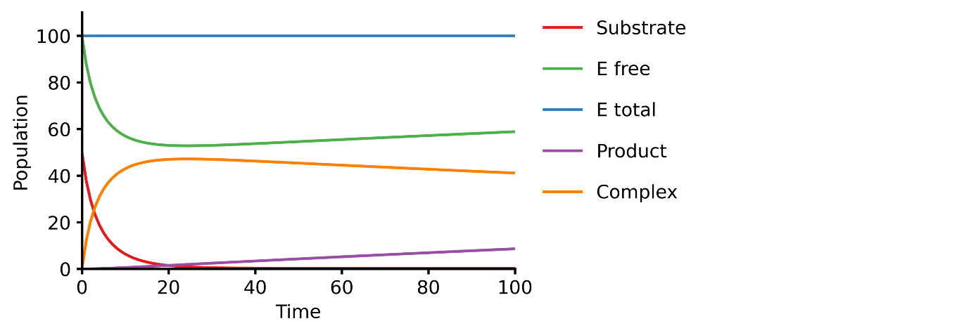
Michaelis-Menten enzyme kinetics

This example shows you how to build a simple Michaelis-Menten two-step enzyme catalysis model with Pasmopy.

E + S ⇄ ES → E + P

An enzyme, E, binding to a substrate, S, to form a complex, ES, which in turn releases a product, P, regenerating the original enzyme.

Prepare a text file describing biochemical reactions (e.g., michaelis_menten.txt)

E + S <--> ES | kf=0.003, kr=0.001 | E=100, S=50
ES --> E + P | kf=0.002

@obs Substrate: u[S]
@obs E_free: u[E]
@obs E_total: u[E] + u[ES]
@obs Product: u[P]
@obs Complex: u[ES]

@sim tspan: [0, 100]

Convert the text into an executable model

$ python

>>> from pasmopy import Text2Model
>>> description = Text2Model("michaelis_menten.txt")
>>> description.convert()
Model information
-----------------
2 reactions
4 species
3 parameters

Run simulation

>>> from pasmopy import create_model, run_simulation
>>> model = create_model("michaelis_menten")
>>> run_simulation(model)

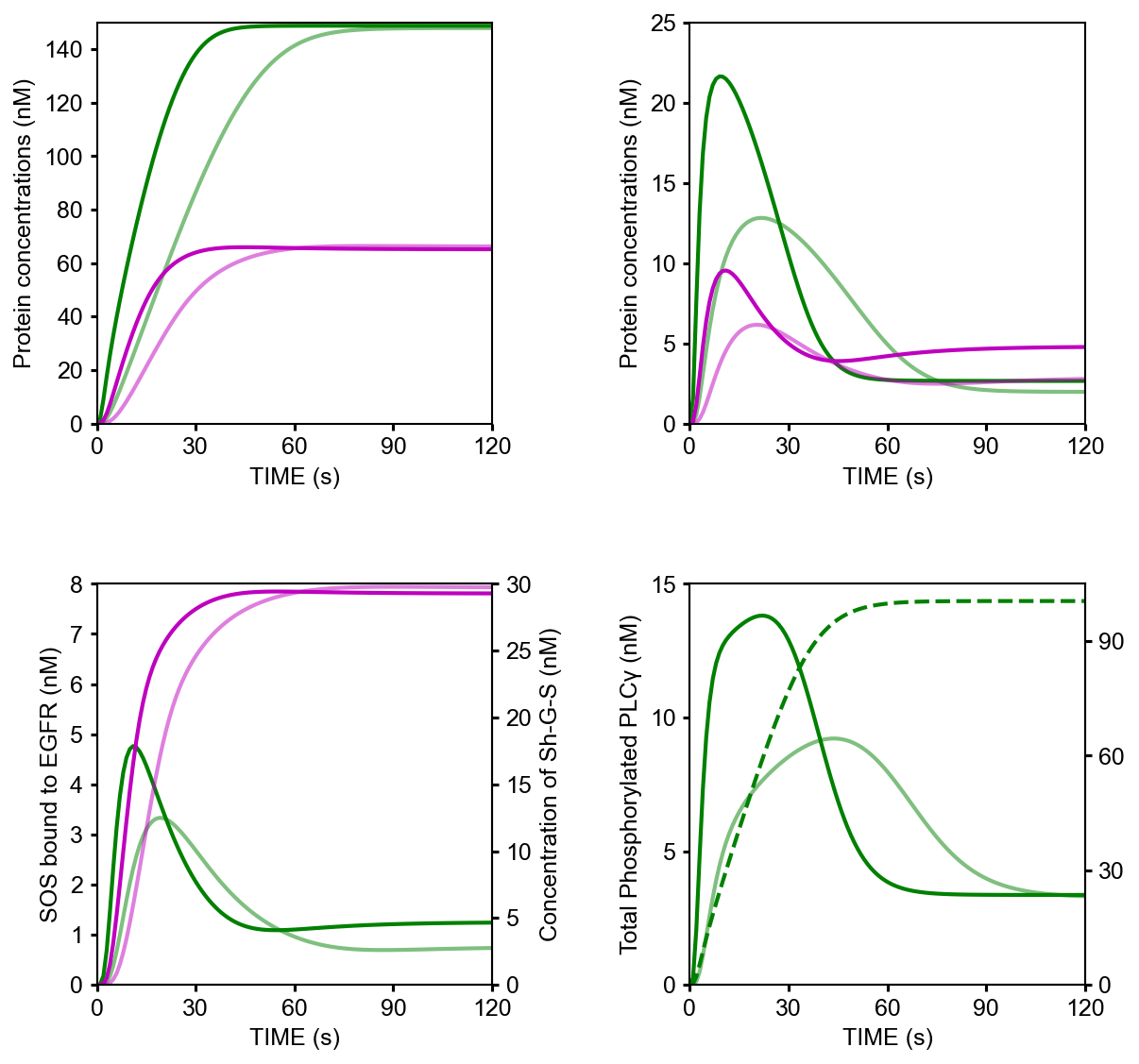
EGF signaling

Below is an example of Pasmopy in action to illustrate EGF signalling pathway.

Reference:

Kholodenko, B. N., Demin, O. V, Moehren, G. & Hoek, J. B. Quantification of short term signaling by the epidermal growth factor receptor. J. Biol. Chem. 274, 30169–30181 (1999). https://doi.org/10.1074/jbc.274.42.30169

Prepare a text describing EGF signaling in hepatocytes (Kholodenko1999.txt)

You can learn how to build the model via Text2Model by comparing the desccription below and the network scheme in Figure 1 in the original paper. The description in the line n denotes the n-th reaction in the scheme.

EGF binds EGFR <--> Ra | kf=0.003, kr=0.06 | EGFR=100
Ra dimerizes <--> R2 | kf=0.01, kr=0.1
R2 is phosphorylated <--> RP | kf=1, kr=0.01
RP is dephosphorylated --> R2 | V=450, K=50
RP binds PLCg <--> RPL | kf=0.06, kr=0.2 | PLCg=105
RPL is phosphorylated <--> RPLP | kf=1, kr=0.05
RPLP is dissociated into RP and PLCgP | kf=0.3, kr=0.006
PLCgP is dephosphorylated --> PLCg | V=1, K=100
RP binds Grb2 <--> RG | kf=0.003, kr=0.05 | Grb2=85
RG binds SOS <--> RGS | kf=0.01, kr=0.06 | SOS=34
RGS is dissociated into RP and GS | kf=0.03, kr=4.5e-3
GS is dissociated into Grb2 and SOS | kf=1.5e-3, kr=1e-4
RP binds Shc <--> RSh | kf=0.09, kr=0.6 | Shc=150
RSh is phosphorylated <--> RShP | kf=6, kr=0.06
RShP is dissociated into ShP and RP | kf=0.3, kr=9e-4
ShP is dephosphorylated --> Shc | V=1.7, K=340
RShP binds Grb2 <--> RShG | kf=0.003, kr=0.1
RShG is dissociated into RP and ShG | kf=0.3, kr=9e-4
RShG binds SOS <--> RShGS | kf=0.01, kr=2.14e-2
RShGS is dissociated into ShGS and RP | kf=0.12, kr=2.4e-4
ShP binds Grb2 <--> ShG | kf=0.003, kr=0.1
ShG binds SOS <--> ShGS | kf=0.03, kr=0.064
ShGS is dissociated into ShP and GS | kf=0.1, kr=0.021
RShP binds GS <--> RShGS | kf=0.009, kr=4.29e-2
PLCgP is translocated to cytoskeletal or membrane structures <--> PLCgP_I | kf=1, kr=0.03

# observable layer
@obs Total_phosphorylated_Shc: u[RShP] + u[RShG] + u[RShGS] + u[ShP] + u[ShG] + u[ShGS]
@obs Total_Grb2_coprecipitated_with_Shc: u[RShG] + u[ShG] + u[RShGS] + u[ShGS]
@obs Total_phosphorylated_Shc_bound_to_EGFR: u[RShP] + u[RShG] + u[RShGS]
@obs Total_Grb2_bound_to_EGFR: u[RG] + u[RGS] + u[RShG] + u[RShGS]
@obs Total_SOS_bound_to_EGFR: u[RGS] + u[RShGS]
@obs ShGS_complex: u[ShGS]
@obs Total_phosphorylated_PLCg: u[RPLP] + u[PLCgP]

# simulation layer
@sim tspan: [0, 120]
@sim condition EGF20nM: init[EGF] = 680
@sim condition EGF2nM: init[EGF] = 68
@sim condition Absence_PLCgP_transloc: init[EGF] = 680; p[kf25] = 0; p[kr25] = 0

Convert the text into an executable model

$ python

To display thermodynamic restrictions, set show_restrictions to True.

>>> from pasmopy import Text2Model
>>> description = Text2Model("Kholodenko_JBC_1999.txt")
>>> description.convert(show_restrictions=True)
Model information
-----------------
25 reactions
23 species
50 parameters

Thermodynamic restrictions
--------------------------
{9, 12, 10, 11}
{15, 18, 21, 17}
{18, 22, 20, 19}
{17, 24, 12, 19}
{23, 24, 20, 15}
{23, 12, 22, 21}

The output of Thermodynamic restrictions shows the cyclic pathways in the biochemical reaction network. These detailed balance relations require the product of the equilibrium constants along a cycle to be equal to 1, since at equilibrium the net flux through any cycle vanishes.

Run simulation

>>> from pasmopy import create_model, run_simulation
>>> model = create_model("Kholodenko_JBC_1999")
>>> run_simulation(model)

Plot simulation results

%matplotlib inline
import os
import matplotlib.pyplot as plt
import numpy as np


def plot_simulation_results(res):

   plt.figure(figsize=(9, 9))
   plt.rcParams['font.family'] = 'Arial'
   plt.rcParams['font.size'] = 12
   plt.rcParams['axes.linewidth'] = 1
   plt.rcParams['lines.linewidth'] = 2

   plt.subplots_adjust(wspace=0.5, hspace=0.4)

   plt.subplot(2, 2, 1)  # ----------------------------------------------------
   for obs_name, color in zip(
      ['Total_phosphorylated_Shc', 'Total_Grb2_coprecipitated_with_Shc'],
      ['g', 'm'],
   ):
      obs_idx = model.observables.index(obs_name)
      for j, condition in enumerate(['EGF20nM', 'EGF2nM']):
            plt.plot(
               model.problem.t,
               res[obs_idx, j],
               color=color,
               alpha=0.5 if condition == 'EGF2nM' else None,
            )
   plt.xlim(0, 120)
   plt.xticks([30*i for i in range(5)])
   plt.ylim(0, 150)
   plt.xlabel("TIME (s)")
   plt.ylabel("Protein concentrations (nM)")

   plt.subplot(2, 2, 2)  # ----------------------------------------------------
   for obs_name, color in zip(
      ['Total_phosphorylated_Shc_bound_to_EGFR', 'Total_Grb2_bound_to_EGFR'],
      ['g', 'm'],
   ):
      obs_idx = model.observables.index(obs_name)
      for j, condition in enumerate(['EGF20nM', 'EGF2nM']):
            plt.plot(
               model.problem.t,
               res[obs_idx, j],
               color=color,
               alpha=0.5 if condition == 'EGF2nM' else None,
            )
   plt.xlim(0, 120)
   plt.xticks([30*i for i in range(5)])
   plt.ylim(0, 25)
   plt.xlabel("TIME (s)")
   plt.ylabel("Protein concentrations (nM)")

   ax1=plt.subplot(2, 2, 3)  # ------------------------------------------------
   ax2 = ax1.twinx()
   for j, condition in enumerate(['EGF20nM', 'EGF2nM']):
      ax1.plot(
            model.problem.t,
            res[model.observables.index('Total_SOS_bound_to_EGFR'), j],
            color='g',
            alpha=0.5 if condition == 'EGF2nM' else None,
      )
      ax2.plot(
            model.problem.t,
            res[model.observables.index('ShGS_complex'), j],
            color='m',
            alpha=0.5 if condition == 'EGF2nM' else None,
      )
   ax1.set_xlim(0, 120)
   ax1.set_xticks([30*i for i in range(5)])
   ax1.set_xlabel("TIME (s)")
   ax1.set_ylim(0, 8)
   ax2.set_ylim(0, 30)
   ax1.set_ylabel("SOS bound to EGFR (nM)")
   ax2.set_ylabel("Concentration of Sh-G-S (nM)")

   ax1=plt.subplot(2, 2, 4)  # ------------------------------------------------
   ax2 = ax1.twinx()
   obs_idx = model.observables.index('Total_phosphorylated_PLCg')
   ax1.plot(
      model.problem.t,
      res[obs_idx, model.problem.conditions.index('EGF20nM')],
      'g',
   )
   ax1.plot(
      model.problem.t,
      res[obs_idx, model.problem.conditions.index('EGF2nM')],
      'g',
      alpha=0.5,
   )
   ax2.plot(
      model.problem.t,
      res[obs_idx, model.problem.conditions.index('Absence_PLCgP_transloc')],
      'g--',
   )
   ax1.set_xlim(0, 120)
   ax1.set_xticks([30*i for i in range(5)])
   ax1.set_ylim(0, 15)
   ax1.set_yticks([5*i for i in range(4)])
   ax1.set_xlabel("TIME (s)")
   ax1.set_ylabel("Total Phosphorylated PLCγ (nM)")
   ax2.set_ylim(0, 105)
   ax2.set_yticks([30*i for i in range(4)])

   plt.show()


if __name__ == '__main__':
   res = np.load(os.path.join(model.path, "simulation_data", "simulations_original.npy"))
   plot_simulation_results(res)

c-Fos expression dynamics

Please refer to https://biomass-core.readthedocs.io/en/latest/tutorial/cfos.html.